Soft Actor-Critic

Although the first soft Actor-Critic (SAC) paper ($\hspace{-0.2em}$ Haarnoja et al., 2018a) dates back to the year 2018, the algorithm remains competitive for model-free Reinforcement Learning (RL) in continuous action spaces. As an off-policy algorithm, SAC can leverage past experience to learn a stochastic policy. SAC was probably the first formulation of an actor-critic algorithm in the maximum entropy (MaxEnt) framework and delivered state-of-the-art results in various benchmarks including robotic tasks ($\hspace{-0.2em}$ Haarnoja et al., 2018b).

The goal of this post is to arrive at a deeper understanding of both, the theoretical derivation and the practical implementation of SAC, which refers to section 4 in the original account ($\hspace{-0.2em}$ Haarnoja et al., 2018a). To this end, we take a detailed look at soft policy iteration, which in a tabular setting will provably converge to the optimal maximum entropy policy. Next, we go through the employed implementation techniques applied to engineer an actor-critic algorithm that is capable of solving practically relevant tasks. To complement the rather theoretical tone, we also deliver a minimal single-file Python implementation of SAC suitable for training RL agents in standard environments provided by the OpenAI Gym benchmark suite ($\hspace{-0.2em}$ Brockman et al., 2016). The code together with checkpoints for training runs in different environments is available via: $\texttt{github.com/chris-hoffmann/post2_soft_actor_critic/tree/main}$

Before we dive into the details of the algorithm, let us start by setting the authors’ contribution in perspective. To this end, we explore the rationale behind the design choices of SAC, compare them with previous approaches, and briefly review recent modifications. In case you would like to skip this introduction and jump right into the main part, please click here.

1. Introduction

1.1 Motivation

SAC is an off-policy actor-critic algorithm that optimizes an entropy-augmented objective. The concept of entropy plays a key role in information theory, thermodynamics, and statistics. Most probability distributions, such as the Gaussian, Geometric, or Pareto distribution, maximize entropy given specific constraints. In other words, these distributions are maximally uniformed (unbiased) towards specific constraints, e.g., a Gaussian is the maximum entropy distribution given a statistic defined by mean and variance. For our purposes, it will be sufficient to treat entropy as a measure of randomness.

In RL, entropy can boost robustness by encouraging the exploration of the joint state-action space as revisiting a small set of state-action pairs repeatedly would result in a low-entropy distribution, which is penalized within the MaxEnt framework. Intuitively, we can interpret the entropy contribution as a regularizer whose role is to fight mode-collapse and over-fitting on collected experience. The latter is similar in spirit to Tikhonov regularization in linear regression, where constraining the L2-norm of the regression coefficients improves generalization by mitigating training set bias. In the popular on-policy PPO algorithm ($\hspace{-0.2em}$ Schulman et al., 2017b), entropy serves a slightly different role by bounding the update of the policy distribution to trustworthy regions of the search space.

A distinct advantage of learning a stochastic policy—as in SAC—is that we can model parity, i.e., the policy can submit similar probability to actions that in a given state yield similar outcomes in terms of reward. The learned policy can also draw from the entire action space since each action has a nonzero probability, which is not the case for algorithms that learn a deterministic policy such as DDPG ($\hspace{-0.2em}$ Lillicrap et al., 2015).

1.2 Related work

Leveraging the MaxEnt framework for RL is an idea that has been explored before ($\hspace{-0.2em}$ Todorov, 2008; $\hspace{-0.2em}$ Fox et al., 2016; $\hspace{-0.2em}$ O’Donoghue et al. 2016; $\hspace{-0.2em}$ Schulman et al., 2017a). The entropy-augmented objective of SAC has, for instance, been applied in the context of inverse RL to learn a reward function from given demonstrations ($\hspace{-0.2em}$ Ziebart et al., 2008).

An earlier paper from the research group of the SAC authors proposed soft Q-Learning, a value-based method that optimizes the same objective as in SAC ($\hspace{-0.2em}$ Haarnoja et al., 2017). While SAC can be seen as a policy-based search formulation, soft Q-Learning recovers the policy from the estimated optimal Q-function. Since the policy distribution is parameterized as an intractable energy model, soft Q-learning involves learning a function approximator to draw samples from the policy. Similar to variational inference, the convergence of soft Q-learning hinges on how well the sampling network approximates the (posterior) policy distribution.

Note that here we use the distinction between policy and value-based methods mainly for pedagogical reasons. In contrast to standard RL, where we optimize for expected return only, both approaches are provably equivalent in the MaxEnt framework ($\hspace{-0.2em}$ Schulman et al., 2017a).

The most related approaches to SAC developed by other research groups, at the time of publication, are likely stochastic value gradients ($\hspace{-0.2em}$ Heess et al., 2015) and trust-PCL ($\hspace{-0.2em}$ Nachum et al., 2017b). Unlike SAC and trust-PCL, the former does not explicitly optimize for a MaxEnt policy. PCL exploits multi-step consistency constraints that hold in the MaxEnt RL framework to jointly learn value function and policy ($\hspace{-0.2em}$ Nachum et al., 2017a). Trust-PCL is a trust region algorithm for off-policy learning in continuous action spaces that builds on PCL. Compared to PCL, confining the degree of the policy change per update step enables trust-PCL to learn more challenging tasks ($\hspace{-0.2em}$ Nachum et al., 2017b), albeit significantly slower than SAC ($\hspace{-0.2em}$ Haarnoja et al., 2018a).

In comparison to previous and concurrent approaches, SAC stood out due to the excellent experimental results in terms of numerical robustness w.r.t. to random initialization, learning speed, and final performance—notably in high-dimensional problems (see panel (f) of Figure 1 in Haarnoja et al., 2018a). Earlier state-of-the-art algorithms for learning in continuous action spaces, such as DDPG ($\hspace{-0.2em}$ Lillicrap et al., 2015), were plagued with poor numerical stability, i.e., training results varied widely across random seeds. The elegant formulation that rests on established textbook knowledge and the later established link to probabilistic inference ($\hspace{-0.2em}$ Levine, 2018) have certainly contributed to the popularity of SAC.

Follow-up work that addressed the overestimation bias ($\hspace{-0.2em}$ Thrun and Schwartz, 1993) to yield more accurate Q-function approximations improved the performance of the SAC algorithm further ($\hspace{-0.2em}$ Kuznetsov et al., 2020; Chen et al., 2021). Another notable line of work extended SAC to enable RL from visual observations in the form of raw pixels ($\hspace{-0.2em}$ Laskin et al., 2020; Yarats et al., 2020).

2. The SAC algorithm

In the following section, we discuss the main concepts of SAC, namely convergence of policy iteration and construction of the deep RL algorithm. We start by introducing standard notation that will be used in the subsequent parts. Note that this account will focus on the newer version of SAC introduced by the original authors ($\hspace{-0.2em}$ Haarnoja et al., 2018b). Compared with the original formulation ($\hspace{-0.2em}$ Haarnoja et al., 2018a), there are two main modifications: (1) we skip learning a separate state-value function, and (2) we add an optimization loop to tune the temperature, which governs the relative impact of reward versus entropy in the objective.

Notation

We can formalize the underlying control problem as policy search in a Markov decision process defined by the tuple $(\mathcal{S}, \mathcal{A}, \mathcal{p}, d_{0}, r, \gamma )$ ($\hspace{-0.2em}$ Sutton & Barto, 2018), where $\mathcal{S}$ is the set of states $s \in \mathcal{S}$, $\mathcal{A}$ is the set of actions $a \in \mathcal{A}$, $\mathcal{p} = p (s_{t+1}|s_{t}, a_{t})$ is the probability for the transition to state $s$ at time $t+1$ by taking action $a_t$ in the previous state $s_t$, $d_{0}$ refers to the initial state distribution at time $t=0$, $r : \mathcal{S} \times \mathcal{A} \rightarrow \mathbb{R}$ defines a reward function for state-action pairs, $\gamma \in (0, 1]$ is a discount factor that down-scales future reward by a constant factor applied at each future time-step. Our goal is to find the policy $\pi$ that optimizes the infinite horizon objective $$ \begin{align*} J(\pi)=\sum_{t=0}^{\infty} \mathbb{E}_{\left(\mathbf{s}_t, \mathbf{a}_t\right) \sim \rho_\pi}\left[\sum_{l=t}^{\infty} \gamma^{l-t} \mathbb{E}_{\mathbf{s}_l \sim p, \mathbf{a}_l \sim \pi}\left[r(\mathbf{s}_t, \mathbf{a}_t)+\alpha \mathcal{H}(\pi(\cdot \vert \mathbf{s}_t)) \vert \mathbf{s}_t, \mathbf{a}_t\right]\right], \tag{1} \end{align*} $$

where state-action pairs are weighted according to the policy-induced distribution $\rho_{\pi}$, $\alpha$ is a temperature factor that controls the relative impact of entropy $\mathcal{H}$. Due to the presence of the entropy term, we explicitly search for a policy that maximizes both, the discounted expected reward and entropy of the policy distribution $\pi(\cdot\vert \mathbf{s}_t)$ for future states conditioned on every state-action pair $(\mathbf{s}_t, \mathbf{a}_t)$ ($\hspace{-0.2em}$ Haarnoja et al., 2018a).

2.1 Soft policy iteration

This section revolves around the convergence proof for the SAC algorithm in the tabular setting. The proof builds on policy iteration, which is a dynamic programming algorithm consisting of two alternating steps: (1) policy evaluation, and (2) policy improvement ($\hspace{-0.2em}$ Sutton & Barto, 2018).

Policy evaluation

Policy evaluation aims to find the state-action value function $Q^\pi: \mathcal{S} \times \mathcal{A} \to \mathbb{R}$ of a given policy by solving the Bellman (expectation) equation iteratively. The underlying convergence that justifies this scheme rests on the contraction mapping theorem ($\hspace{-0.2em}$ Kreyszig, 1991). Following this established line of argumentation, the SAC authors propose a soft Bellman operator $\mathcal{T}$ that acts on the space of bounded real-valued soft $Q$-functions $Q \in \mathcal{Q}$ by mapping $\mathcal{T}: \mathcal{Q} \to \mathcal{Q}$, $$ \begin{align*} \mathcal{T} Q(\mathbf{s}_t, \mathbf{a}_t) & \triangleq \,r(\mathbf{s}_t, \mathbf{a}_t)+\gamma \mathbb{E}_{\mathbf{s}_{t+1} \sim p}\left[V(\mathbf{s}_{t+1})\right] \tag{2} \\
& \overset{(i)}{=} \,r(\mathbf{s}_t, \mathbf{a}_t) + \gamma \mathbb{E}_{\mathbf{s}_{t+1} \sim p}\big[\mathbb{E}_{\mathbf{a}_{t+1} \sim \pi}\left[Q(\mathbf{s}_{t+1}, \mathbf{a}_{t+1})-\alpha \log (\pi(\mathbf{a}_{t+1} \vert \mathbf{s}_{t+1}))\right]\big] \\
& \overset{(ii)}{=} \underbrace{r(\mathbf{s}_t, \mathbf{a}_t)+ \gamma \alpha \mathbb{E}_{\mathbf{s}_{t+1} \sim p}\left[\mathcal{H}(\pi\left(\cdot \vert \mathbf{s}_{t+1})\right)\right]} + \gamma \mathbb{E}_{\mathbf{s}_{t+1} \sim p, ,\mathbf{a}_{t+1} \sim \pi}\left[Q(\mathbf{s}_{t+1}, \mathbf{a}_{t+1})\right] \nonumber \\
& = \hspace{5em} r_\pi( \mathbf{s}_t, \mathbf{a}_t, \mathbf{s}_{t+1}) \hspace{4em} + \gamma \mathbb{E}_{\mathbf{s}_{t+1} \sim p, ,\mathbf{a}_{t+1} \sim \pi}\left[Q(\mathbf{s}_{t+1}, \mathbf{a}_{t+1})\right]. \tag{3} \end{align*} $$

Note that in step ($i$), we define the soft state value function $$ \begin{align*} V(\mathbf{s}_{t+1}) = \mathbb{E}_{\mathbf{a} \sim \pi} \big[Q(\mathbf{s}_{t+1}, \mathbf{a}_{t+1}) - \alpha\log(\pi(\mathbf{a}_{t+1} \vert \mathbf{s}_{t+1}))\big]. \tag{4} \end{align*} $$

In step ($ii$), we exploit the definition of (differential) entropy, $\mathcal{H}(f) = \mathbb{E}[-\log(f(X))]$, where $X$ refers to a random variable from sample space $\mathcal{X}$ with probability density function $f$.

Given the definition of $\mathcal{T}$, we can write the Bellman equation in compact notation $$ \begin{align*} Q_{k+1}(\mathbf{s}, \mathbf{a}) = [\mathcal{T},Q_k](\mathbf{s}, \mathbf{a}) = [\mathcal{T}_k,Q_0](\mathbf{s}, \mathbf{a}), \tag{5} \end{align*} $$

where $k$ refers to the $k$-th application of $\mathcal{T}$ and $Q_0$ denotes the initial estimate. We can show that $\mathcal{T}$ is a contraction mapping on $\mathcal{Q}$ w.r.t. the maximum norm $\Vert Q \Vert_\infty = \max\limits_{\mathbf{s},\mathbf{a}} Q$ $$ \begin{align*} \Vert \mathcal{T}Q_2 -\mathcal{T}Q_1 \Vert_\infty \leq \gamma \Vert Q_2 - Q_1\Vert_\infty \qquad\; \forall Q_2, Q_1 \in \mathcal{Q}. \tag{6} \end{align*} $$

As $\gamma$ is bounded to $[0, 1)$, intuitively this means that the mapping performed by $\mathcal{T}$ shrinks the distance between $Q_2$ and $Q_1$, effectively bringing their images closer together. Note that in the derivation above, we need to restrict the action and state space to be finite, i.e., $\vert \mathcal{A} \vert < \infty$ and $\vert \mathcal{S} \vert < \infty$, to ensure that $r_\pi$ is bounded.

Since $\mathcal{Q}$ spans a complete metric space, it follows that $\mathcal{T}$ is bounded and has a unique fixed point. We can prove this proposition by exploiting the fact that the Cauchy sequence $(Q_k)$ converges to a fixed point that lies in $\mathcal{Q}$. While the exact derivation of the proof is presented elsewhere ($\hspace{-0.2em}$ Kreyszig, 1991; $\hspace{-0.2em}$ Szepesvári, 2010), a key consequence for us is that we can approximate the fixed point of $\mathcal{T}$ by repeatedly applying a contraction mapping. The comparison with the Bellman equation from above ($\hspace{-0.2em}$ Equation 5) reveals that the fixed point indeed coincides with the soft state-action value function of the given policy since $Q^{\pi} = \lim_{k \rightarrow \infty} \mathcal{T}_k Q_0$.

Policy improvement

Policy improvement is step 2 of the policy iteration algorithm in which we leverage the state-action value function obtained from policy evaluation.

In the standard formulation, where we optimize for the expected return only, we update the policy estimate by acting greedy, i.e., $\pi_{\text{new}}=\underset{\pi’}{\arg \max } \;Q^{\pi_{\text {old}}}(s_t, \pi’(\cdot \vert s_t))$. A nice result of this update rule is that our policy estimate will be strictly improving and converge to the optimal policy ($\hspace{-0.2em}$ Sutton & Barto, 2018). Following this chain of thought, the SAC authors propose the following update rule for the entropy-augmented objective $$ \begin{equation*} \pi_{\text {new }}=\arg \min _{\pi^{\prime}} \mathrm{D}_{\mathrm{KL}}\bigg(\pi^{\prime}(\cdot \vert \mathbf{s}_t) \,\Bigg|\!\Bigg|\, \frac{\exp (\frac{1}{\alpha} Q^{\pi_{\text {old}}}(\mathbf{s}_t, \cdot))}{Z^{\pi_{\text {old }}}(\mathbf{s}_t)}\bigg) \tag{7} \end{equation*} $$

and show that this rule yields a strictly improving policy in the MaxEnt framework. The actual proof presented next is largely retrieved from the original paper ($\hspace{-0.2em}$ Haarnoja et al., 2018a). A few hints and comments were added for easier understanding.

Applying the definition of the Kuhlback-Leibler divergence, $\mathrm{D}_{\mathrm{KL}}(P\Vert Q)=\int _{{-\infty }}^{{\infty }}p(x)\cdot \log\big({\frac{p(x)}{q(x)}}\big)\;{\mathrm d}x$, we reformulate the update rule as follows: $$ \begin{align*} \pi_{\text{new}}&=\arg \min _{\pi^{\prime}} \mathbb{E}_{\mathbf{a}_t \sim \pi\prime}\Biggl[\log \Biggl(\frac{\pi^{\prime}(\cdot \vert \mathbf{s}_t)}{\exp (\frac{1}{\alpha} Q^{\pi_{\text {old}}}(\mathbf{s}_t, \cdot)) \frac{1}{Z^{\pi_{\text{old}}}(\mathbf{s}_t)}}\Biggr)\Biggr] \nonumber \\
&=\arg \min _{\pi^{\prime}} \mathbb{E}_{\mathbf{a}_t \sim \pi\prime}\Bigl[ \log (\pi^{\prime}(\cdot \vert \mathbf{s}_t)) - \tfrac{1}{\alpha}Q^{\pi_{\text{old}}}(\mathbf{s}_t, \cdot) + \log(Z^{\pi_{\text{old}}}(\mathbf{s}_t)) \Bigr] \nonumber \\
& =\arg \min _{\pi^{\prime}} J_{\pi_{\text{old}}}(\pi^{\prime}(\cdot \vert \mathbf{s}_t)). \end{align*} $$

Since $\pi_{\text{new}}$ is the argument that minimizes the objective $J_{\pi_{\text{old}}}$, it holds that $$ \begin{align*} J_{\pi_{\text{old}}}(\pi_{\text{new}}(\cdot \vert \mathbf{s}_t)) &\leq J_{\pi_{\text{old}}}(\pi_{\text{old }}(\cdot \vert \mathbf{s}_t)) \tag{9} \\
\mathbb{E}_{\mathbf{a}_{\mathbf{t}} \sim \pi_{\text{new}}}\bigl[\log (\pi_{\text{new}}(\mathbf{a}_t \vert \mathbf{s}_t))-\tfrac{1}{\alpha}Q^{\pi_{\text{old}}}(\mathbf{s}_t, \mathbf{a}_t)+\log(Z^{\pi_{\text {old}}}(\mathbf{s}_t))\bigr] &\leq \mathbb{E}_{\mathbf{a}_{\mathbf{t}} \sim \pi_{\text{old}}}\bigl[\log(\pi_{\text{old}}(\mathbf{a}_t \vert \mathbf{s}_t))-\tfrac{1}{\alpha}Q^{\pi_{\text{old}}}(\mathbf{s}_t, \mathbf{a}_t)+\log(Z^{\pi_{\text{old}}}(\mathbf{s}_t))\bigr] \nonumber \\
\mathbb{E}_{\mathbf{a}_t \sim \pi_{\text{new}}}\bigl[Q^{\pi_{\text{old}}}(\mathbf{s}_t, \mathbf{a}_t)-\alpha\log(\pi_{\text{new}}(\mathbf{a}_t \vert \mathbf{s}_t))\bigr] &\geq V^{\pi_{\text{old}}}(\mathbf{s}_t). \tag{10} \end{align*} $$

Note that in the last step, we exploit the fact that the partition function $Z^{\pi_{\text{old}}}(\mathbf{s}_t)$ is independent of action $\mathbf{a}_t$. Substituting the obtained inequality into the Bellman equation, we can show that the updated policy $\pi_\text{new}$ is indeed an improvement: $$ \begin{align*} Q^{\pi_{\text{old}}}(\mathbf{s}_t, \mathbf{a}_t) & = r_t + \gamma \mathbb{E}_{\mathbf{s}_{t+1} \sim p}[V^{\pi_{\text{old}}}(\mathbf{s}_{t+1})] \nonumber \\
& \leq r_t +\gamma \mathbb{E}_{\mathbf{s}_{t+1} \sim p}\big[\mathbb{E}_{\mathbf{a}_{t+1} \sim \pi_{\text {new}}}[Q^{\pi_{\text{old}}}(\mathbf{s}_{t+1}, \mathbf{a}_{t+1})- \alpha\log (\pi_{\text{new}}(\mathbf{a}_{t+1} \vert \mathbf{s}_{t+1}))]\big] \nonumber \\
&\overset{(i)}{=} r_t + \gamma \mathbb{E}_{\mathbf{s}_{t+1} \sim p}\Big[\mathbb{E}_{\mathbf{a}_{t+1} \sim \pi_{\text{new}}}\big[r_{t+1} + \gamma \mathbb{E}_{\mathbf{s}_{t+2} \sim p}[V^{\pi_{\text{old}}}(\mathbf{s}_{t+2})]- \alpha\log(\pi_{\text{new}}(\mathbf{a}_{t+1} \vert \mathbf{s}_{t+1}))\big]\Big] \nonumber \\
& \leq r_t + \gamma \mathbb{E}_{\mathbf{s}_{t+1} \sim p}\Big[\mathbb{E}_{\mathbf{a}_{t+1} \sim \pi_{\text{new}}}\big[r_{t+1} + \gamma \mathbb{E}_{\mathbf{s}_{t+2} \sim p}[Q^{\pi_{\text{old}}}(\mathbf{s}_{t+2}, \mathbf{a}_{t+2})-\alpha\log(\pi_{\text{new}}(\mathbf{a}_{t+2} \vert \mathbf{s}_{t+2}))]-\alpha\log(\pi_{\text{new}}(\mathbf{a}_{t+1} \vert \mathbf{s}_{t+1}))\big]\Big] \nonumber \\
& \;\;\vdots \nonumber \\
&= \mathbb{E}_{\mathbf{s} \sim p, \mathbf{a} \sim \pi_{\text{new}}} \bigg[\sum_{t=0} \gamma^t r_t + \alpha \sum_{t=1} \gamma^t \log(\pi_{\text{new}}(\mathbf{a}_t\vert\mathbf{s}_t))\bigg] \nonumber \\
& \leq Q^{\pi_{\text{new}}}(\mathbf{s}_t, \mathbf{a}_t). \tag{11} \end{align*} $$

Note that here and hereinafter we employ the shorthand notation $r_{t} = r(\mathbf{s}_t, \mathbf{a}_t)$. In step $(i)$, we expand $Q^{\pi_{\text{old}}}(\mathbf{s}_{t+1}, \mathbf{a}_{t+1})$ according to the Bellman equation ($\hspace{-0.2em}$ Equation 2). We apply this expansion, in ascending order, at each time step followed by plugging in Inequality 10, which eventually yields $Q^{\pi_{\text{new}}}$.

Policy iteration

In the previous section, we looked at how to obtain better policies w.r.t. to our maximum entropy objective by updating our estimate according to Equation 7. We concluded that the updated policy $\pi_{\text{new}}$ is indeed better or equal to any previous estimate. To find the state-action value function of $\pi_{\text{new}}$, we can then resort to policy evaluation. Afterwards, we perform another policy improvement step, i.e., we compute the exponential of the $Q$-function and update the policy ($\hspace{-0.2em}$ Equation 7). Through this policy iteration scheme of alternating between evaluation and improvement steps, we obtain a sequence of improving policies (and $Q$-functions). Since the action space and the state space are finite, so is the number of policies. Hence, the algorithm will provably converge in a finite number of steps. From deriving the policy improvement, we know that for the converged policy $\pi^*$ the value of the objective $J_{\pi^*}$ of any other policy $\pi$ must be lesser or equal than $J_{\pi^*}(\pi^*)$ ($\hspace{-0.2em}$ Equation 9) and equivalently that $ Q^{\pi^*}\!(\mathbf{s}_t, \mathbf{a}_t) \geq Q^{\pi}(\mathbf{s}_t, \mathbf{a}_t) \;\; \forall (\mathbf{s}_t, \mathbf{a}_t) \in \mathcal{S} \times \mathcal{A}$ ($\hspace{-0.2em}$ Equation 11). Hence, $\pi^*$ is indeed the optimal policy.

We remind that the presented convergence proof for soft policy iteration is constrained to the tabular setting, where the state-action space is small enough to fit into memory. For a practically relevant actor-critic algorithm, we approximate the soft $Q$-function and policy $\pi$ with neural networks to map state-action pairs to expected (entropy-augmented) return and to output the policy parameters, respectively. Unlike in policy iteration, we skip running policy evaluation and improvement to convergence. Instead, we optimize these networks jointly using stochastic gradient descent. In practice, it is common to restrict the policy estimates to be spherical Gaussian distributions. Speaking of implementation details, this will be the theme of the next section. Before taking a deep dive into how to construct the SAC algorithm in practice, let us briefly reflect on the rule for updating the policy by minimizing the difference between the current policy and the Boltzmann-like distribution with the exponential of the $Q$-function in the numerator, which corresponds to the reference distribution in Equation 7. Yes, we have seen that the math works out nicely, i.e., this update rule results in a monotonic improvement of the policy estimate. Also true, we can interpret this reference distribution as an energy model. Still, the motivation for this particular update rule feels a bit arbitrary. In follow-up work, the last author of the SAC papers presents a detailed derivation through the lens of probabilistic inference ($\hspace{-0.2em}$ Levine, 2018). Interested in a few more details? Then please take a look at the Appendix located at the bottom of the page. Interested in all the details, then it is probably a good idea to check out the original source ($\hspace{-0.2em}$ Levine, 2018).

2.2 Derivation of the Soft Actor-Critic algorithm

Let us now study how to implement soft policy iteration as a deep RL algorithm. To this end, actor $\pi$ and critic $Q$ are parameterized using neural networks, and we rely on stochastic gradient descent to optimize the parameters of both networks in parallel.

Critic Update

The update rule for learning the soft state-action value function is inspired by Q-learning, i.e., we aim to minimize the mean squared difference between LHS and RHS of the Bellman expectation equation ($\hspace{-0.2em}$ Equation 2). To this end, we rely on minibatches $ \begin{align*} \mathcal{B} =\{(\mathbf{s}_{t}, \mathbf{a}_{t}, r_{t}, \mathbf{s}_{t+1})_j\}_{j=1}^{k} \end{align*} $ comprising of $k$-tuples uniformly drawn from a replay buffer $D$ that stores data from past rollouts. Importantly, the actions $\mathbf{a}_{t+1}$ are not sampled from the replay buffer as this would reflect the choice of a policy that is likely to be outdated. To improve the current estimate of the state-action value function, we therefore need to sample from the latest policy estimate $\tilde{\pi}$ to compute $Q^{\pi}(\mathbf{s}_{t+1}, \mathbf{a}_{t+1})$.

In practice, we rely on two additional techniques for stabilizing training:

1. To decouple action selection from action evaluation, we employ target networks $\widehat{Q}$ in the calculation of the targets, i.e., the RHS of the Bellman equation. The parameters of the target networks $\widehat{\theta}$ are the exponential moving average of the soft $Q$-function parameters, $\widehat{\theta} = \tau , \theta + (1 - \tau),\widehat{\theta}$, where $0 < \tau < 1$, and $\tau$ refers to the mixing coefficient that is typically chosen to be close to $0$ ($\approx 5.0\cdot10^{-3}$).
2. We apply a clipped-double $Q$-scheme ($\hspace{-0.2em}$ Fujimoto et al., 2018) to mitigate optimism bias in the target prediction ($\hspace{-0.2em}$ Thrun and Schwartz, 1993). This means we learn two independent $Q$-functions $Q_{\theta_i}$, where $i \in {1,2}$, that share the same network architecture, and use the minimum, i.e., the more conservative estimate to compute the targets.

Taken together, we arrive at the following objective $J_Q$ for learning the soft $Q$-functions: $$ \begin{equation*} J_Q(\theta_i; \mathcal{B}) = \mathbb{E}_{\mathcal{B}\sim \mathcal{U}(D)} \Biggl[ \frac{1}{2}\biggl(Q_{\theta_i}(\mathbf{s}_t, \mathbf{a}_t) - \underbrace{\Bigl(r_t + \gamma \Big[\min_{i=1,2}\widehat{Q}_{\widehat{\theta}_i}(\mathbf{s}_{t+1}, \tilde{\mathbf{a}}_{t+1}) - \alpha\log({\pi(\tilde{\mathbf{a}}_{t+1} \vert \mathbf{s}_{t+1}}))\Big]}_{=y(r_t,\: \mathbf{s}_{t+1},\: \tilde{\mathbf{a}}_{t+1})} \Bigr)\biggr)^{2}\Biggr], \tag{12} \end{equation*} $$

where $ \begin{align*} \tilde{\mathbf{a}}_{t+1} \sim \tilde{\pi} \end{align*} $ is sampled from the latest policy estimate and $y(r_t, \mathbf{s}_{t+1}, \tilde{\mathbf{a}}_{t+1})$ refers to the targets.

We optimize this objective using stochastic gradient descent thereby approximating the gradient as follows: $$ \begin{equation} \nabla_{\theta_i} J_Q(\theta_i; \mathcal{B}) = \mathbb{E}_{\mathcal{B}\sim \mathcal{U}(D)} \big[ (Q_{\theta_i}(\mathbf{s}_t, \mathbf{a}_t) - y(r_t, \mathbf{s}_{t+1}, \tilde{\mathbf{a}}_{t+1}))~\nabla_{\theta_i}Q_{\theta_i}(\mathbf{s}_t, \mathbf{a}_t)\big]. \tag{13} \end{equation} $$

Actor Update

The actor network approximates $\pi$ as a Gaussian distribution specified by mean and diagonal covariance. To update the network parameters $\phi$ during training, we can directly minimize the KL divergence in Equation 7. Exploiting the definition of the KL divergence yields the following objective $$ \begin{equation} J_\pi(\phi; D) = \hspace{-1em} \underset{\substack{ \quad \mathbf{s}_t \sim \mathcal{U}(D) \\ \,\mathbf{a}_t \sim \pi_{\phi}}}{\mathbb{E}}\big[\alpha \log (\pi_\phi(\mathbf{a}_t \vert \mathbf{s}_t)) - \min _{i=1,2} Q_{\theta_i}(\mathbf{s}_t, \mathbf{a}_t)\big], \tag{14} \end{equation} $$

where we approximate the expectations in the policy objective with samples. For the expectation under states, we sample a minibatch from the replay buffer. For the expectation under actions, we rely on single sample estimates from the policy distribution. Note that we have omitted the ($\log$ of the) partition function in Equation 14 since it is a normalization constant that lacks a contribution to the gradient of the policy objective.

In general, we have two principles of choice for maximizing the objective $J_\pi$ as a function of the policy parameters $\phi$. As in the REINFORCE algorithm ($\hspace{-0.2em}$ Williams, 1992), we could rely on the likelihood ratio gradient estimator, which frees us from backpropagating through the policy network. However, this option often results in high-variance gradient estimates and hence poor convergence. Alternatively, we can resort to option number two in which we apply the re-parameterization trick to deal with the fact that in our objective we have $ \mathbb{E}_{\mathbf{a} \sim \pi_{\phi}} $. In other words, our expectation over actions depends implicitly on the network parameters $\phi$ that we aim to optimize. Without this dependency, we could evaluate the expectation of the gradient as the gradient of the expectation, i.e., $\nabla_{\phi}\mathbb{E}_{\mathbf{a} \sim q}\left[ u_{\phi}(\mathbf{a})\right] = \mathbb{E}_{\mathbf{a} \sim q}\left[\nabla_{\phi} u_{\phi}(\mathbf{a})\right]$, where $u$ is an arbitrary function of $\mathbf{a}$ parameterized by $\phi$. In this example, the actions are drawn from a distribution $q$ that is *independent* of $\phi$. We can eliminate the cumbersome implicit dependency by applying the following reparameterization: We express the actions as values of a differentiable function $f_{\phi}: \mathcal{S} \to \mathcal{A}$, $\mathbf{a}_t = f_{\phi}(\mathbf{\epsilon}_t; \mathbf{s}_t)$, where $\mathbf{\epsilon}$ is a random input vector drawn from a normal distribution $\mathcal{N}(\mathbf{0},\mathbf{I})$. Due to this transformation, which corresponds to the change of a random variable, we can obtain actions by sampling $\mathbf{\epsilon}$ and then evaluating $f_{\phi}(\mathbf{\epsilon}_t; \mathbf{s}_t)$. As a consequence, our expectation is no longer under actions but under the random vector that conveniently is independent of $\phi$, i.e., $\mathbb{E}_{\mathbf{\epsilon}_t \sim \mathcal{N}}$. As sketched above, we can thus compute the gradient of the expectation as the expectation of the gradient, which permits us to update the policy estimate via gradient ascent. To this end, we rely on the following gradient estimator derived by applying the chain rule for total derivatives: $$ \begin{equation} \nabla_{\phi} J_\pi(\phi, f_\phi; D) = \nabla_{\phi} J_\pi(\phi, f_\phi) + \nabla_{f_\phi} J_\pi(\phi, f_\phi)\nabla_\phi f_\phi. \tag{15} \end{equation} $$

To compute this gradient, we see that we need to differentiate the actions w.r.t. the network parameters ($\nabla_\phi f_\phi$), which is a consequence of the reparameterization. From a practical point of view, this is straightforward to implement when relying on auto-differentiation engines such as Tensorflow ($\hspace{-0.2em}$ Abadi et al., 2016) or PyTorch ($\hspace{-0.2em}$ Paszke et al., 2019) as they provide reparameterizable distribution functions amenable to gradient-based parameter optimization. Taken together, we arrive at the gradient estimator $$ \begin{equation} \nabla_{\phi} J_{\pi}(\phi; D) = \hspace{-1em} \underset{\substack{\quad \mathbf{s}_t \sim \mathcal{U(D)} \\ \!\mathbf{\epsilon}_t \sim \mathcal{N}}}{\mathbb{E}}\big[\alpha \log(\pi_\phi(\tilde{\mathbf{a}}_t \vert \mathbf{s}_t)) - \min _{i=1,2} Q_{\theta_i}(\mathbf{s}_t, \tilde{\mathbf{a}}_t)\big]. \tag{16} \end{equation} $$

As in the critic update, we use the more conservative $Q$-function evaluation and obtain actions from the current policy estimate.

Action bounds

Our policy is a parameterized Gaussian distribution of infinite range, which is not acceptable for numerical experiments. To bound the range of the action values to the finite interval $(-1, +1)$, we apply hyperbolic tangent to the Gaussian samples with corresponding probability density $f(\mathbf{x}|\mathbf{s}) \sim \mathcal{N}$, $\mathbf{a} = \tanh(\mathbf{x})$, where $\mathbf{x} \in \mathbb{R}^{|\mathcal{A}|}$ denotes a vector of random variables that is of the same dimension as the action space.

This transformation of random variables, by applying $\tanh$ element-wise, permits us to compute the log-likelihood of actions in closed form $$ \begin{equation} \log (\pi(\mathbf{a} \vert \mathbf{s})) = \log \biggl(f(\mathbf{x} \vert \mathbf{s})\left|\operatorname{det}\left(\frac{\mathrm{d} \mathbf{a}}{\mathrm{d} \mathbf{x}}\right)\right|^{-1}\biggr) =\log (f(\mathbf{x}\vert\mathbf{s}))-\sum_{i=1}^{|\mathcal{A}|} \log\big(1-\tanh ^2(x_i)\big), \tag{17} \end{equation} $$

where we used $ \frac{\mathrm{d} \mathbf{a}}{\mathrm{d} \mathbf{x}}=\operatorname{diag}\left(1-\tanh ^2(\mathbf{x})\right) $ and $x_i$ denotes the $i$-th component of $\mathbf{x}$. This expression can suffer from poor numerical stability since the argument of the $\log$ can be evaluated to zero when $\tanh(\mathbf{x})$ is rounded to $1$ due to low numerical precision. To improve numerical stability, we replace the problematic term as follows: $1-\tanh ^2(x) = \operatorname{sech}^2(x) = 2 \left( \log(2) - x - \operatorname{softplus}(-2x)\right)$, where $\operatorname{softplus}(x) = \log(1+\exp(-x))$ ($\hspace{-0.2em}$ Yarats et al., 2020). While we apply the $\operatorname{softplus}$ trick in the provided code, we abstain from integrating additional modifications ($\hspace{-0.2em}$ Bjorck et al., 2021) to improve numerical stability even further. Combining the reparameterization trick and $\tanh$-transformation, we end up with the following expression for drawing actions from policy $\pi$: $$ \begin{align*} \mathbf{a}_{t; \phi}(\mathbf{s}_t, \mathbf{\epsilon}_t) = \tanh\bigl( \mu_{\phi}(\mathbf{s}_t) + \sigma_{\phi}(\mathbf{s}_t) \odot \mathbf{\epsilon}_t\bigr). \tag{18} \end{align*} $$

Optimization of the entropy contribution

The first SAC paper ($\hspace{-0.2em}$ Haarnoja et al., 2018a) demonstrated that learning is rather stable across random seeds chosen for parameter initialization. However, training success depends strongly on the numerical value of the temperature $\alpha$, which controls the relative contribution of the entropy term in the policy objective, thereby balancing exploration (high entropy) vs. exploitation (low entropy and therefore a high impact of the reward term). Hence, it is no surprise that the optimal temperature appears to be a key and task-specific hyperparameter. In the second SAC paper ($\hspace{-0.2em}$ Haarnoja et al., 2018b), the authors present a scheme for adjusting the temperature during training by formulating policy search as a constrained optimization problem to maximize expected return while satisfying a minimum entropy constraint $\mathcal{H}_0$: $$ \begin{align*} \max _{\pi_{0: T}} \mathbb{E}_{\rho_\pi}\Bigg[\sum_{t=0}^T r_t\Bigg] \text { s.t. } \underbrace{\mathbb{E}_{(\mathbf{s}_t, \mathbf{a}_t) \sim \rho_\pi}\big[-\log (\pi_t(\mathbf{a}_t \vert \mathbf{s}_t))\big]}_{\mathcal{H}(\pi_t)} \geq \mathcal{H}_0 \qquad \forall t, \tag{19} \end{align*} $$

where heuristically $ \begin{align*} \mathcal{H}_0 \end{align*} $ is set to the negative dimension of the action space, i.e., $\mathcal{H}_0 = - |\mathcal{A}|$. Since the policy at time step $t$ only influences the future time steps $t+1:T$, we can find the optimal sequence $\pi_{0:T}$ via dynamic programming. This involves proceeding back in time—starting at $T$—to optimize $\pi_t$ recursively. We can formulate the Lagrangian $\mathcal{L}$ for the constraint optimization (at a particular time step $t$) as follows: $$ \begin{align*} \mathcal{L}(\pi_t, \lambda_t) = \mathbb{E}_{\rho_\pi}\big[r_t\big] + \lambda_t( \mathcal{H}(\pi_t) - \mathcal{H}_0). \tag{20} \end{align*} $$

The comparison with the (undiscounted) policy objective ($\hspace{-0.2em}$ Equation 1) shows that the Lagrange multiplier (or dual variable) $\lambda$ controls the relative contribution of the entropy term. Hence, we can interpret this variable as temperature $\alpha$. Exploiting strong duality, we express the dual problem as $$ \begin{align*} \max _{\pi_t} \mathbb{E}_{\left(\mathbf{s}_t, \mathbf{a}_t\right) \sim \rho_\pi}\!\left[r_t\right]=\min _{\alpha_t \geq 0} \max _{\pi_t} \mathbb{E}\left[r_t-\alpha_t \log (\pi_t(\mathbf{a}_t \vert \mathbf{s}_t))\right]-\alpha_t \mathcal{H}_0. \tag{21} \end{align*} $$

To solve this problem, we can perform dual gradient descent, which involves maximizing the primal variable $\pi^*$ (as well as $Q^*$—details omitted) followed by solving the dual variable $\alpha_t^*$ according to $$ \begin{align*} \alpha_t^*=\arg \min _{\alpha_t} \mathbb{E}_{\mathbf{a}_t \sim \pi_t^*}\left[-\alpha_t \log (\pi_t^*(\mathbf{a}_t \vert \mathbf{s}_t ; \alpha_t)) - \alpha_t \mathcal{H}_0\right]. \tag{22}
\end{align*} $$

For more details, please consult the original account ($\hspace{-0.2em}$ Haarnoja et al., 2018b). Here, we limit the exposition to a sketch of the main theoretical ideas since in practice a rather heuristic approach is taken to optimize the temperature jointly with the policy and soft $Q$-function: Dropping the time-dependency, we learn a single temperature parameter by optimizing the objective $$ \begin{equation} J_\alpha(D) = \hspace{-1em} \underset{\substack{\quad \mathbf{s}_t \sim \mathcal{U(D)} \\ \,\mathbf{a}_t \sim \pi_{\phi}}}{\mathbb{E}}\big[-\alpha \log (\pi(\tilde{\mathbf{a}}_t \vert \mathbf{s}_t))-\alpha \mathcal{H}_0 \big]. \tag{23} \end{equation} $$

Intuitively, this objective results in an increase (decrease) in temperature when the entropy of the policy estimate is lower (higher) than the minimum expected entropy.

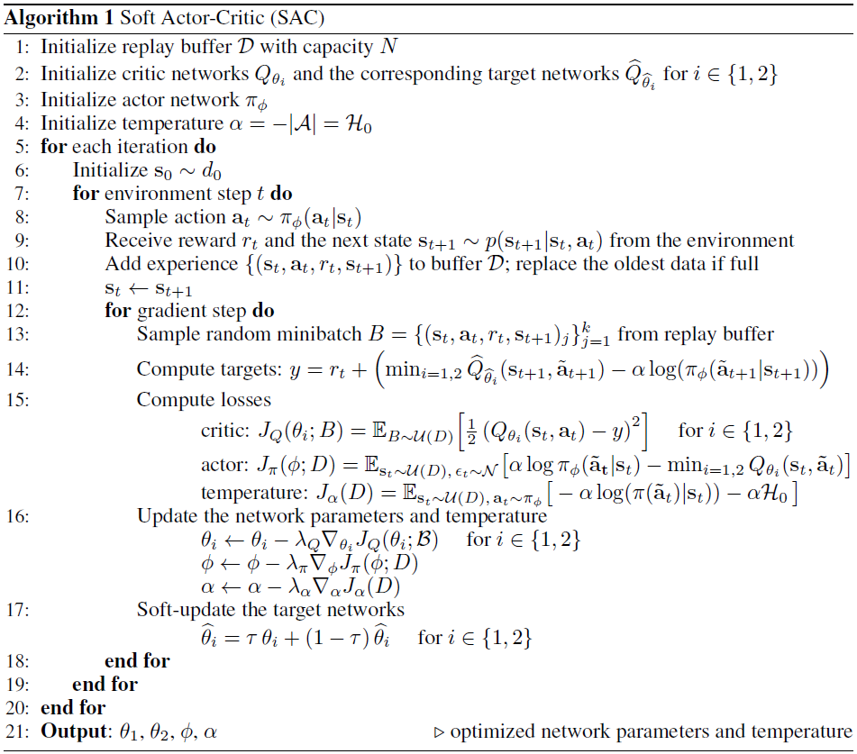
This brings us to the end of the implementation section. In Algorithm 1, we summarize the various steps of the SAC algorithm. For demonstration purposes, we translate the algorithm into Python code thereby relying on PyTorch ($\hspace{-0.2em}$ Paszke et al., 2019) as the engine for automatic differentiation. We leverage our implementation to train SAC agents in 3 different environments with continuous action spaces (HalfCheetah, InvertedPendulum, Hopper) available in the openAI Gym benchmark suite ($\hspace{-0.2em}$ Brockman et al., 2016). The code together with training curves and model checkpoints is available via: $\texttt{github.com/chris-hoffmann/post2_soft_actor_critic/tree/main}$

References

• Abadi, M., Barham, P., Chen, J., Chen, Z., Davis, A., Dean, J., … and Zheng, X. (2016). TensorFlow: Large-Scale Machine Learning on Heterogeneous Distributed Systems. arXiv preprint arXiv:1603.04467.
• Bjorck, J., Chen, X., De Sa, C., Gomes, C. P., Weinberger, K. (2021). Low-Precision Reinforcement Learning: Running Soft Actor-Critic in Half Precision. In International Conference on Machine Learning (ICML).
• Brockman, G., Cheung, V., Pettersson, L., Schneider, J., Schulman, J., Tang, J., & Zaremba, W. (2016). OpenAI Gym. arXiv preprint arXiv:1606.01540.
• Chen, X., Wang, C., Zhou, Z., Ross, K. (2021). Randomized Ensembled Double Q-Learning: Learning Fast Without a Model. arXiv preprint arXiv:2101.05982.
• Fox, R., Pakman, A., Tishby, N. (2016). Taming the noise in reinforcement learning via soft updates. arXiv preprint arXiv:1512.08562.
• Fujimoto, S., van Hoof, H., Meger, D. (2018). Addressing Function Approximation Error in Actor-Critic Methods. arXiv preprint arXiv:1802.09477.
• Haarnoja, T., Tang, H., Abbeel, P., Levine, S. (2017). Reinforcement Learning with Deep Energy-Based Policies. In International Conference on Machine Learning (ICML).
• Haarnoja, T., Zhou, A., Abbeel, P., Levine, S. (2018a). Soft Actor-Critic: Off-Policy Maximum Entropy Deep Reinforcement Learning with a Stochastic Actor. In International Conference on Machine Learning (ICML).
• Haarnoja, T., Zhou, A., Hartikainen, K., Tucker, G., Ha, S., Tan, J., Kumar, V., Zhu, H., Gupta, A., Abbeel, P., Levine, S. (2018b). Soft Actor-Critic Algorithms and Applications. arXiv preprint arXiv:1812.05905.
• Heess, N., Wayne, G., Silver, D., Lillicrap, T., Erez, T., Tassa, Y. (2015). Learning Continuous Control Policies by Stochastic Value Gradients. In Advances in Neural Information Processing Systems (NeurIPS).
• Kreyszig, E. (1991). Introductory Functional Analysis with Applications (Vol. 17). John Wiley & Sons.
• Kuznetsov, A., Shvechikov, P., Grishin, A., Vetrov, D. (2020). Controlling Overestimation Bias with Truncated Mixture of Continuous Distributional Quantile Critics. In International Conference on Machine Learning (ICML).
• Laskin, M., Srinivas, A., Abbeel, P. (2020). CURL: Contrastive Unsupervised Representations for Reinforcement Learning. In International Conference on Machine Learning (ICML).
• Levine, S. (2018). Reinforcement Learning and Control as Probabilistic Inference: Tutorial and Review. arXiv preprint arXiv:1805.00909.
• Lillicrap, T. P., Hunt, J. J., Pritzel, A., Heess, N., Erez, T., Tassa, Y., Silver, D., Wierstra, D. (2015). Continuous control with deep reinforcement learning. arXiv preprint arXiv:1509.02971
• Nachum, O., Norouzi, M., Xu, K., Schuurmans, D. (2017a). Bridging the Gap Between Value and Policy Based Reinforcement Learning. In Advances in Neural Information Processing Systems (NeurIPS).
• Nachum, O., Norouzi, M., Xu, K., Schuurmans, D. (2017b). Trust-PCL: An Off-Policy Trust Region Method for Continuous Control. arXiv preprint arXiv:1707.01891.
• O’Donoghue, B., Munos, R., Kavukcuoglu, K., Mnih, V. (2016). PGQ: Combining policy gradient and Q-learning. arXiv preprint arXiv:1611.01626.
• Paszke, A., Gross, S., Massa, F., Lerer, A., Bradbury, J., Chanan, G., … and Chintala, S. (2019). PyTorch: An Imperative Style, High-Performance Deep Learning Library. In Advances in Neural Information Processing Systems (NeurIPS).
• Schulman, J., Abbeel, P., Chen, X. (2017a). Equivalence Between Policy Gradients and Soft Q-Learning. arXiv preprint arXiv:1704.06440.
• Schulman, J., Wolski, F., Dhariwal, P., Radford, A., Klimov, O. (2017b). Proximal Policy Optimization Algorithms. arXiv preprint arXiv:1707.06347.
• Sutton, R. S. and Barto, A. G. (2018). Reinforcement Learning: An introduction (2nd ed.). MIT Press.
• Szepesvári, C. (2010). Algorithms for Reinforcement Learning. Morgan & Claypool Publishers.
• Thrun, S. and Schwartz, A. (1993). Issues in Using Function Approximation for Reinforcement Learning. In Proceedings of the Fourth Connectionist Models Summer School.
• Todorov, E. (2008). General Duality between Optimal Control and Estimation. In Conference on Decision and Control (CDC).
• Williams, R. J. (1992). Simple statistical gradient-following algorithms for connectionist reinforcement learning. Machine learning, 8, 229-256.
• Yarats, D., Kostrikov, I., Fergus, R. (2020). Image Augmentation Is All You Need: Regularizing Deep Reinforcement Learning from Pixels. In International Conference on Learning Representations (ICLR).
• Ziebart, B. D., Maas, A., Bagnell, J. A., Dey, A. K. (2008). Maximum Entropy Inverse Reinforcement Learning. In International Conference on Artificial Intelligence (AAAI).

Appendix: Control as probabilistic inference

The update rule for the policy, i.e., minimizing the difference between the current policy and the Boltzmann-like distribution ($\hspace{-0.2em}$ Equation 7) in which the Q-function serves as a negative energy can also be motivated through the lens of probabilistic modeling. In follow-up work, the senior author of the SAC papers presented a thorough derivation of the proposed rule motivated by a probabilistic graphical model ($\hspace{-0.2em}$ Levine, 2018). The hidden Markov-like model contains special nodes $\mathcal{O}_t$ for encoding the optimal action as a boolean variable, where the probability of the optimal action at time step $t$, $p(\mathcal{O}_t = 1 \vert \mathbf{s}_t, \mathbf{a}_t)$ is equal to $\exp{(\frac{1}{\alpha}r_t)}$. By conditioning on the optimal trajectory $\tau \triangleq (\mathbf{s}_0, \mathbf{a}_0, \dots, \mathbf{s}_T, \mathbf{a}_T)$, we can infer the most probable action distribution. In essence, we cast policy optimization as probabilistic inference.

Derivation

The goal is to determine the policy that minimizes the difference between a candidate distribution $p_{\pi_\phi}(\tau) = p(\mathbf{s}_0) \prod_{t=0}^{T} p(\mathbf{s}_{t+1} \vert \mathbf{s}_t, \mathbf{a}_t)\pi_\phi(\mathbf{a}_t \vert \mathbf{s}_t)$ and the optimal trajectory distribution $p(\tau \vert \mathcal{O}_{0:T} = 1)\propto p(\mathbf{s}_0) \prod_{t=0}^{T} p(\mathbf{s}_{t+1} \vert \mathbf{s}_t, \mathbf{a}_t)\exp{\left(\sum_{t=0}^{T} \frac{1}{\alpha}r_t\right)}$: $$ \begin{align} D_{\mathrm{KL}}(p_{\pi_\phi}(\tau) | p(\tau \vert \mathcal{O}_{0:T} = 1))= & -E_{p_{\pi_\phi}(\tau)} \left[\log(p(\tau \vert \mathcal{O}_{0:T} =1)) - \log(p_{\pi_\phi}(\tau)) \right] \nonumber \\
= & -\mathbb{E}_{p_{\pi_\phi}(\tau)} \left[\log(p(\mathbf{s}_0))+\sum_{t=0}^T\left(\log(p(\mathbf{s}_{t+1} \vert \mathbf{s}_t, \mathbf{a}_t))+\frac{1}{\alpha}r_t\right)\right. \nonumber \\
& -\left.\log (p(\mathbf{s}_0))-\sum_{t=0}^T\bigg(\log (p(\mathbf{s}_{t+1} \vert \mathbf{s}_t, \mathbf{a}_t))+\log (\pi_{\phi}(\mathbf{a}_t \vert \mathbf{s}_t))\bigg)\right] \nonumber \\
= & -\mathbb{E}_{p_{\pi_\phi}(\tau)}\left[\sum_{t=0}^T r_t-\alpha\log(\pi_\phi(\mathbf{a}_t \vert \mathbf{s}_t))\right] \nonumber \\
= & -\sum_{t=0}^T \mathbb{E}_{(\mathbf{s}_t, \mathbf{a}_t) \sim p_{\pi_\phi}(\mathbf{s}_t, \mathbf{a}_t)}\left[r_t-\alpha\log(\pi_\phi(\mathbf{a}_t \vert \mathbf{s}_t))\right] \nonumber \\
= & -\sum_{t=0}^T \mathbb{E}_{(\mathbf{s}_t, \mathbf{a}_t) \sim p_{\pi_\phi}(\mathbf{s}_t, \mathbf{a}_t)}\left[r_t\right]+\alpha\mathbb{E}_{\mathbf{s}_t \sim p_{\pi_\phi}(\mathbf{s}_t)}\left[\mathcal{H}(\pi_\phi(\cdot \vert \mathbf{s}_t))\right]. \tag{A1} \end{align} $$

Since the KL-divergence is non-negative and zero iff the candidate distribution is the optimal distribution, we see that the optimal policy maximizes the expected return and the expected entropy of the policy distribution.

We can optimize Equation A1 via recursion by employing a dynamic programming scheme. In other words, starting with the base case at the final step $T$, we move backward in time to find the optimal policy. In this context, let us examine the recursive case. For a given time step $t$, we aim to maximize the sum of two terms that represent the contribution of the current time and all subsequent time steps, respectively: $$ \begin{align*} & \mathbb{E}_{(\mathbf{s}_t, \mathbf{a}_t) \sim p_{\pi_\phi}(\mathbf{s}_t, \mathbf{a}_t)}\big[r_t-\alpha\log(\pi_\phi(\mathbf{a}_t \vert \mathbf{s}_t))\big]+\mathbb{E}_{\left(\mathbf{s}_t, \mathbf{a}_t\right) \sim p_{\pi_\phi}\left(\mathbf{s}_t, \mathbf{a}_t\right)}\big[\mathbb{E}_{\mathbf{s}_{t+1} \sim p_{\pi_\phi}(\mathbf{s}_{t+1} \vert \mathbf{s}_t, \mathbf{a}_t)}[V(\mathbf{s}_{t+1})]\big] = \nonumber \\
& \mathbb{E}_{\mathbf{s}_t \sim p_{\pi_\phi}(\mathbf{s}_t)} \Bigl[\mathbb{E}_{\mathbf{a}_t \sim \pi_\phi} \bigl[-\alpha\log(\pi_\phi(\mathbf{a}_t \vert \mathbf{s}_t)) + r_t + \mathbb{E}_{\mathbf{s}_{t+1} \sim p_{\pi_\phi}(\mathbf{s}_{t+1} \vert \mathbf{s}_t, \mathbf{a}_t)} [V(\mathbf{s}_{t+1})]\bigr]\Bigr] = \nonumber \\
& \mathbb{E}_{\mathbf{s}_t \sim p_{\pi_\phi}(\mathbf{s}_t)} \Bigl[-\mathbb{E}_{\mathbf{a}_t \sim \pi_\phi} \bigl[+\log(\pi_\phi(\mathbf{a}_t \vert \mathbf{s}_t)) - \tfrac{1}{\alpha}Q(\mathbf{s}_t, \mathbf{a}_t) + \log(Z( \mathbf{s}_t))\bigr] \Bigr] + \log(Z( \mathbf{s}_t)) = \nonumber \\
& \mathbb{E}_{\mathbf{s}_t \sim p_{\pi_\phi}(\mathbf{s}_t)}\bigg[-D_{\mathrm{KL}}\bigg(\pi_\phi(\mathbf{a}_t \vert \mathbf{s}_t) \,\Bigg|\!\Bigg|\, \frac{\exp (\frac{1}{\alpha}Q(\mathbf{s}_t, \mathbf{a}_t))}{Z(\mathbf{s}_t)} \bigg)+\log(Z(\mathbf{s}_t))\bigg], \tag{A2} \end{align*} $$

where we have applied the definition of $Q$ ($\hspace{-0.2em}$ Equation 2). Further, we can connect the state value function to the partition function since $$ \begin{align*} V(\mathbf{s}_t) & = \log(Z(\mathbf{s}_t)) = \log\bigg(\int_{\mathcal{A}} \exp (\tfrac{1}{\alpha}Q(\mathbf{s}_t, \mathbf{a}_t))\, \mathrm{d}\mathbf{a}_t\bigg). \tag{A3} \end{align*} $$

It is straightforward to show that the base case $t=T$ yields the same result as in the recursive case. We can therefore conclude that our recursive scheme resembles solving the Bellman equation with the difference that here the state value function is computed as a soft maximum (in $\log$ space). We can then leverage the optimal $Q$ and state value function to obtain the optimal policy since $ \pi_\phi(\mathbf{a}_t \vert \mathbf{s}_t)=\exp (\frac{1}{\alpha}Q(\mathbf{s}_t, \mathbf{a}_t)-V(\mathbf{s}_t))$ minimizes the KL-divergence in Equation A2 (and Equation 7).

Beyond the tabular setting or when dealing with continuous action spaces, we can still use function approximation to optimize a lower variational bound of this objective. As in the standard RL problem, we can thereby rely on policy-gradient methods or actor-critic formulations ($\hspace{-0.2em}$ Levine, 2018).